How to plot the Gamma function fractal

The Gamma function is an extension of the factorial (n!) function, with its argument shifted down by 1, to real and complex numbers. And there is a fractal associated to it. I just wanted to learn how to make it because I want to learn how to plot the Mandelbrot set, and the Gamma function fractal seems easier to catch the idea of recursion. So here is how to make it!

First of all, I have been following the great explanation at Mathistopheles website, but I needed to study by myself some details to make it work properly.  

Basically, when the gamma function is calculated for a complex number z repeatedly (nested, and shifting down 1 the complex number according to the definition), this is: Gamma(Gamma(...(Gamma(z-1)...-1)-1), the final value result of the nested calculations either tends to 1 or grows without limit. So it is possible to map each z (=a+bi) value of the complex plane (in Cartesian coordinates) with a color code showing if the value tends to 1 (this the same as saying that it tends to the complex number 1+0i) or not in a specific numbers of calculations of the nested Gamma function. 

The condition to tend to 1 is as follows: let us say we want to know if the nested calculation of the Gamma function applied to z = (a+bi) tends to 1. In a first step, calculate Gamma(z-1) = c+di. If the distance of the real part a to 1 is greater or equal to the distance of c to 1 and the absolute value of the imaginary part b is greater than the absolute value of the imaginary part d (abs(b)>=abs(d)) then it is possible to say that z tends to 1+0i when the Gamma function is applied over z (nested as it was explained above). 

It is important to understand that it can happen that the first calculation for a given complex number z1 of Gamma(z1-1) provides a complex number z2 which is not closer to 1 than the original z1. And that does not mean that z1 does not tend to 1 when the nested Gamma function is applied again to z2. It could happen that when Gamma(z2-1) = z3 is calculated, z3 is closer to 1 than z2, and in the moment that this happens then the result is that from that point z1 tends to 1 when the nested calculations are applied. So sometimes we just need one calculation of Gamma for the initial complex number z1 to know if it tends to 1 and sometimes we need two nested Gamma calculations, sometimes 3, 4, 5, ... etc sometimes hundreds or thousands. But the calculation of the computer is very slow when the Gamma function is applied hundreds of times for each complex number, so usually a limit of for instance 7 nested Gamma calculations is applied to decide if a complex number tends to 1 or not. It is not totally accurate, but good enough to start to see the fractal patterns of the Gamma function. The more nested calculations the more accurate the patterns will be, and of course, the more complex numbers are calculated, the more we can zoom into the fractal pattern. 

And here is the result:

It is the typical image of the Gamma fractal function in the complex plane interval [-5,0]+[-1,1]i. I tried to find a good combination of colors. The complex numbers that tend to 1 in just one Gamma calculation are in black color. Then Dark blue two nested calculations, then Pink... finally up to Yellow (7 nested loops). The complex numbers that do not tend to 1 in less than 8 nested calculations are in the Blue color (if the reader can rememeber the good old Fractint, it was the popular color used for that purpose!).

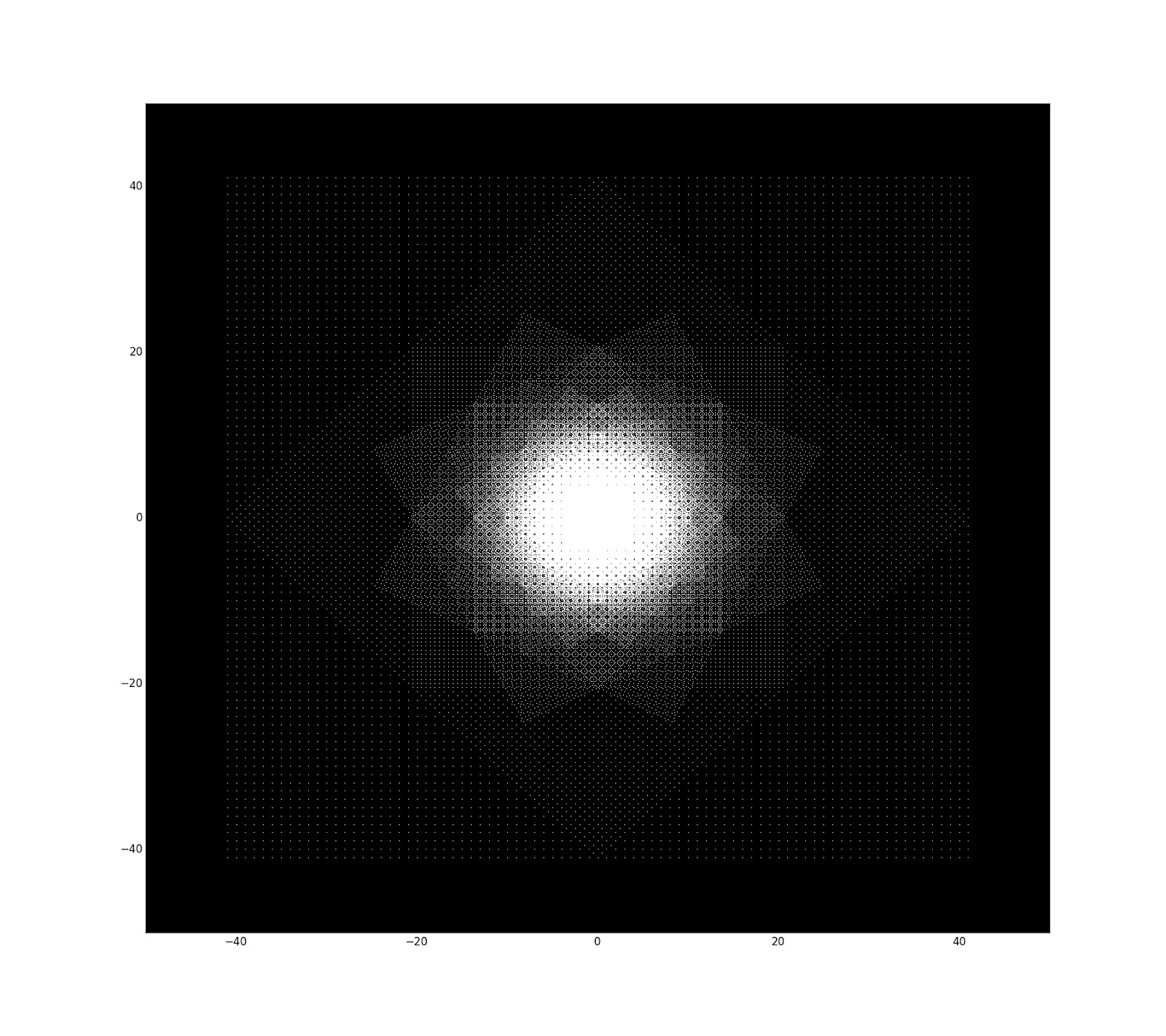
Just to finish here is another version in polar coordinates:

And here is the Python code, modifying the value of the "method" variable it is possible to render Cartesian, Polar or Spherical coordinates. Use it freely:

def gamma_fractal():
    import matplotlib.pyplot as plt
    from scipy.special import gamma
    from numpy import real, imag, around, arange, float, cos, sin, pi

    import matplotlib as mpl

    from mpl_toolkits.mplot3d import Axes3D

   
    #0 Cartesian, 1 Polar, 3 Spherical
    method = 0

    if method==3:
        mpl.rcParams['legend.fontsize'] = 10


        fig = plt.figure()

        ax = fig.gca(projection='3d')
       
    arraydim = 1000000
    xrange = [arange(arraydim,dtype=float),arange(arraydim,dtype=float),arange(arraydim,dtype=float),arange(arraydim,dtype=float),arange(arraydim,dtype=float),arange(arraydim,dtype=float),arange(arraydim,dtype=float),arange(arraydim,dtype=float)]
    yrange = [arange(arraydim,dtype=float),arange(arraydim,dtype=float),arange(arraydim,dtype=float),arange(arraydim,dtype=float),arange(arraydim,dtype=float),arange(arraydim,dtype=float),arange(arraydim,dtype=float),arange(arraydim,dtype=float)]
    zrange = [arange(arraydim,dtype=float),arange(arraydim,dtype=float),arange(arraydim,dtype=float),arange(arraydim,dtype=float),arange(arraydim,dtype=float),arange(arraydim,dtype=float),arange(arraydim,dtype=float),arange(arraydim,dtype=float)]
    hexcolor=["#000000","#131667","#F028B3","#42677C","#3EA670","#6DD02D","#F9B90F","#0000FF"]
    pos=[0,0,0,0,0,0,0,0]
   
    ival = 0+1j

    if method!=3:
        firstx = -5
        lastx = 0
        firsty = -1
        lasty = 1
        incx = 0.0005
        incy = 0.0005
    else:
        firstx = -pi
        lastx = pi
        firsty = -pi
        lasty = pi
        incx = 0.002
        incy = 0.002
    posx = firstx
   
   
    while posx < lastx:
        posy = firsty
        while posy < lasty:
            counter = 0           
            mycomplex = gamma((posx+1)+(posy*ival))
            nextcomplex = gamma(mycomplex+1)

            while counter < 7:
                if (abs(mycomplex.imag) > abs(nextcomplex.imag)) and (abs(1-mycomplex.real) > abs(1-nextcomplex.real)):
                    break
                mycomplex = nextcomplex
                nextcomplex = gamma(mycomplex+1)

                counter = counter + 1
           
            if method == 0:
                xrange[counter][pos[counter]] = posx
                yrange[counter][pos[counter]] = posy
            elif method == 1:
                xrange[counter][pos[counter]] = posx*cos(posy)
                yrange[counter][pos[counter]] = posx*sin(posy)
            else:
                xrange[counter][pos[counter]] = cos(posy)*cos(posx)
                yrange[counter][pos[counter]] = sin(posy)*cos(posx)
                zrange[counter][pos[counter]] = sin(posx)

            pos[counter] = pos[counter] + 1

            if pos[counter]==arraydim:
                newxrange = arange(pos[counter],dtype=float)       
                newyrange = arange(pos[counter],dtype=float)
                newzrange = arange(pos[counter],dtype=float)   

                for i in range(0,pos[counter]):
                    newxrange[i]=xrange[counter][i]
                    newyrange[i]=yrange[counter][i]
                    if method == 3:
                        newzrange[i]=zrange[counter][i]

                if method != 3:
                    plt.plot(newxrange,newyrange,",",color=hexcolor[counter])
                else:
                    ax.plot(newxrange, newyrange, newzrange,",",color=hexcolor[counter])


                pos[counter]=0
           
            posy = posy + incy
        posx = posx + incx

    for c in range (0,8):
        newxrange = arange(pos[c],dtype=float)       
        newyrange = arange(pos[c],dtype=float)       
        newzrange = arange(pos[c],dtype=float)   
        for i in range(0,pos[c]):
            newxrange[i]=xrange[c][i]
            newyrange[i]=yrange[c][i]
            if method == 3:
                newzrange[i]=zrange[c][i]

        if method != 3:
            plt.plot(newxrange,newyrange,",",color=hexcolor[c])
        else:
            ax.plot(newxrange, newyrange, newzrange,",",color=hexcolor[c])

           
        pos[c]=0

    if method!=3:
        ax = plt.gca()
        ax.set_axis_bgcolor((0, 0, 0))
        figure = plt.gcf()
        figure.set_size_inches(30, 20)
        if method == 0:
            plt.axis([firstx,lastx,firsty,lasty])
        plt.savefig("gamma_"+str(method)+".png")
        plt.show()
    else:
        #ax.legend()
        #ax.dist=8
        for ii in range(0,361):
            ax.view_init(elev=-178., azim=ii)
            mpl.pyplot.savefig("movie"+str(ii)+".png")
        #ax.view_init(elev=28., azim=ii)
        #plt.show()


gamma_fractal()

Enjoy the fractals!

A very nice pattern based on Euler's identity

Euler's identity is one of the jewels of Mathematics, it blends in one sight some of the most significant constants of the mathematical universe:

I tried to visualize how would look the left part of the identity in the complex plane by using the following function:

It is a tryout of a generic version of the left side of Euler's identity. Applying the change e^{ib}=cos(b)+sin(b)i, the following function is obtained:

For instance, to be able to see the patterns, taking k1,k2,k3 in the interval [−10,10] stepping in by 0.1, and calculating all the possible combinations of triplets (k1,k2,k3) and their values f(k1,k2,k3), this is the pattern that it generates when the complex values a+bi are represented in Cartesian coordinates (a=x,b=y):

A closer approach to 0+0i:

Euler's identity f(1,1,1)=e^{pi*i}+1=0+0i would be located at the center and the rest of points are the closer values of the more generic function f(k1,k2,k3) as it was defined above for the example. As expected is periodic and symmetrical. This is a little video:

Isn't it hypnotic? I have asked at MSE about this pattern, as far as I know it might be the fist time that has been plotted. I hope somebody will be able to propose some insights about it!  

Update 2016/01/15: Professor Brent Yorgey kindly gave a very nice explanation of the pattern at MSE!

About the similarities between the patterns found on the Complex Division and some Quasicrystal diffraction patterns

As the brilliant and wise professor William Thurston said: "Mathematics is an art of human understanding. … Our brains are complicated devices, with many specialized modules working behind the scenes to give us an integrated understanding of the world. Mathematical concepts are abstract, so it ends up that there are many different ways they can sit in our brains. A given mathematical concept might be primarily a symbolic equation, a picture, a rhythmic pattern, a short movie — or best of all, an integrated combination of several different representations."

In the case of the following test, the concepts are pictures and movies. As in my former post regarding the patterns that can be found in the roots of quadratic and cubic equations, I wanted to know if there are patterns hidden in the complex division, and it seems I found some interesting too!  

Indeed, reviewing the results of my former post, and thanks to the kind insights from the administrator of the Number Theory group in LinkedIn, it seems that they look like the patterns of the refraction of some type of quasicrystal structures. Are they related? I do not know, but so far here is what I have found:

1. First this is the description of the test:  the images are showing the set S of complex numbers a+bi represented in the Cartesian plane (a=x, b=y) obtained from the divisions of the complex numbers: z1/z2 , where z1 = (A+Ai) and z2 =  (B+Bi) being A and B natural numbers both of the interval [-41..41]. The set S contains all the possible combinations of divisions between z1 and z2 in those intervals (except when z2=0+0i which is not represented). Then a zoom is applied to show only a zoomed part of the whole pattern.

2. As the intervals used for the test are the same ones, A = B = [-41..41], this is the original lattice or mesh of complex numbers that will be divided between the whole same mesh of complex numbers (every point of this image represents a complex number and the output of the test is the division of each one of those complex numbers by all the complex numbers of the mesh)

3. This is a zoom-out to see the result of the complex division. This is the complete set S seen from the interval x=y=[-50,50]. As it can be seen in the image, due to the complex division formula, different meshes representing different subsets of the complex division are generated rotating on the center 0+0i. Up to the interval x=y=[-1..1], the closer we are to the center, the more different meshes are swapped, and the denser it is the quantity of complex numbers of the set. For smaller intervals inside x=y=[-1..1] (e.g. x=y=[-0.5,0.5]) the closer we get to the center (I will call it nucleus too) the darker it gets. The peak of density is at x=y=[-1..1], so the image is brighter when it is zoomed on that interval. Clicking in the image it is possible to see details on the structures that are generated due to the swapping of the meshes. They are similar to tessellations.

4. This is a zoom-in in the frame x,y in [-1.2,1.2]. There is symmetry in both axis, X and Y.

5. Zooming-in even more, it is possible to see how it looks like the nucleus near 0+0i, this is x,y in [-0.1,0.1]. The more meshes are swapped the more interesting patterns appear. The image below is obtained by using the intervals A=B=[-81..81] instead of A=B=[-41..41] because the closer we get into the center inside x=y=[-1..1] the darker it is, so it is required a bigger set S to have more density and bright (so the pattern closer to the nucleus is easier to see).

Summarizing, the following video shows a zoom-in, zoom-out into the patterns that can be seen in the set of complex numbers obtained from the divisions of the complex numbers: z1/z2 , where z1 = (A+Ai) and z2 =  (B+Bi) where A and B are natural numbers in the interval [-41..41]. The set generates all the possible combinations of divisions between z1 and z2 in those intervals.

So far those are the results of the test. Now, what similarities can be found between those images and the refraction patterns of quasicrystals? Let us compare. 

1. Something basic,  credits to the Wikipedia, this is the X-ray diffraction pattern of the natural Al₆₃Cu₂₄Fe₁₃ quasicrystal.

2. Credits to Steffen Weber, this is a simulation of diffraction pattern, which could represent either electron diffraction patterns or the zeroth layers of precession photographs (X-ray), dodecagonal QC:  

The pattern above looks similar to the zoom-in in the pattern of the complex division for the interval x=y=[-1..1]. I suspect that the complex division produces those patterns due to a n-fold rotational symmetry. See here for more information too.

3. Credits to Damian OHara. More refraction patterns:

4. In this link there is a very good technical description of the refraction patterns. And in this link there are more examples of n-fold symmetries. In this one there are similar star-like patterns as the ones I found at the roots of quadratic equations.

So far this is all I have found. I will try to look for more information, but at least the similarities are quite interesting.

I would like to finish this post with two of the best videos I found about quasicrystal, tesselations and tiling. The first one is from Sir Roger Penrose, "Forbidden crystal symmetry in mathematics and architecture".

And my favorite one! Professor Marjorie Senechal, "Quasicrystals Gifts to Mathematics":

Please if somebody reading this knows more about the subject let me know, I would like to learn more about it.

Hobbymath's wanderings #11

"Dancing with Fractals: The Chaos Game (With Music!)"(pdf).

"Remainders of Square Numbers (Youtube).

Sounding Number: Chaos Game.

Introduction to Algebraic Topology (Youtube).

Heath-Brown’s theorem on prime twins and Siegel zeroes.

Gamma function (Wiki).

Mathistopheles: Fractal Factorials.

Gaussian Primes.

The Complex Tale of Eisenstein Prime Numbers.

Benford's Very Strange Law (YouTube).

Battle of Eigenvalues of al most periodic matrices (YouTube).

Polymath and the gap between primes (YouTube).

Billiards and moduli spaces (YouTube).

Curtis McMullen on "Manifolds, Topology and Dynamics" (YouTube).

Julia Set (Wiki).

A Century of Complex Dynamics.

Fractal patterns and Chaos Game by prof. Robert L. Devaney.

Cantor and Sierpinski, Julia and Fatou: Complex Topology Meets Complex Dynamics, by prof. Robert L. Devaney.

Fractal Factorials (about Gamma function fractal in complex plane).

Landau Lectures| Prof. Thurston 1995/6 (YouTube).

Visualizing the patterns in the sets of complex and real roots of quadratic and cubic equations

This is an extension of a question I did at MSE: "What methods are known to visualize patterns in the set of real roots of quadratic equations?".

I came across a previous awesome question about the visualization of the distribution of polynomial roots and tried to do a simpler version applied first to the set of real roots of quadratic equations ax^2+bx+c=0 and then to cubic equations ax^3+bx^2+cx+d=0 to visualize the complex roots (meaning all the roots of the equation represented as complex numbers) and only the real roots (a subset of the complex roots when the imaginary part is zero).

To visualize the pattern of the relationship between the set of roots of the quadratic equations, I prepared a Python program to calculate the roots x1,x2 only for the specific values of the intervals a in [−ai,ai], b in [−bi,bi], c in [−ci,ci], a,b,c are natural numbers N. If the limits ai,bi,ci are very big, the set of roots is very dense and it is very difficult to visualize the emerging pattern.

Complex roots of quadratic equations in Cartesian coordinates (x = real part of the root, y = imaginary part of the root). ai=bi=ci=75:

Complex roots of quadratic equations represented in polar coordinates (theta = real part of the root, r = imaginary part of the root). ai=bi=ci=65:

Real roots (subset of the complex roots whose imaginary part is zero) of quadratic equations represented in Cartesian coordinates (x,y)=(x1,x2). E.g. ai,bi,ci=75:

This is an special subset: real roots (subset of the complex roots whose imaginary part is zero) of quadratic equations whose coefficients are irrational numbers, when ai,bi,ci=575 and using only the square roots of the prime numbers of those intervals, sqrt(a)/a in [−ai,ai], sqrt(b)/b in [−bi,bi], sqrt(c)/c in [−ci,ci]. This will show the pattern of the roots only for a) a,b,c irrationals (because the square roots of prime numbers are irrational numbers) and still constrained to b) x1,x2 in R:

Real roots (subset of the complex roots whose imaginary part is zero) of quadratic equations represented in polar coordinates (theta,r)=(x1,x2). E.g. ai,bi,ci=75:

Due to the symmetries the opposite patterns (x,y)=(x2,x1) and (theta,r)=(x2,x1) are similar.

Real roots (subset of the complex roots whose imaginary part is zero) of quadratic equations represented in spherical coordinates (theta,phi,r)=(x1,x2,1). E.g. ai,bi,ci=25:

Here is an animation (it will take a little bit to upload, please be patient)

So basically there seems to be a pattern in the relationship between both real roots that can be visualized.

Here is the same exercise for the three roots (x1,x2,x3) of the cubic equations. 

Complex roots of cubic equations represented in Cartesian coordinates (the x value is the real value and the y value is the imaginary value):

Complex roots of cubic equations represented in polar coordinates, (theta, r), each root will be represented by the angle theta = real part of the root and the radius r = the imaginary part of the root.

Representing the real roots requires more imagination because there are three real roots and is possible to play with the symmetry of the roots.

Real roots (subset of the complex roots whose imaginary part is zero) of cubic equations represented in Cartesian coordinates (x,y)=(x1,x2),(x1,x3),(x2,x3),(x2,x1),(x3,x1),(x3,x2). E.g. ai,bi,ci=25:

Real roots (subset of the complex roots whose imaginary part is zero) of cubic equations represented in polar coordinates (theta,r)=(x1,x2),(x1,x3),(x2,x3),(x2,x1),(x3,x1),(x3,x2). E.g. ai,bi,ci=20:

Finally, the real roots (subset of the complex roots whose imaginary part is zero) of cubic equations represented in spherical coordinates (theta,phi,r)=(x1,x2,1),(x2,x3,1),(x1,x3,1),(x2,x1,1),(x3,x2,1),(x3,x1,1). E.g. ai,bi,ci=25:

I would like to learn other methods to visualize the sets of roots and would appreciate very much any feedback about this subject.