A similar conjecture to Fortunate numbers based on sum of the divisors of n

The last months of 2015 I have been trying to get more expressions similar to the ones I found in my previous post "About Fortunate numbers and other similar expressions". So this is a follow-up note with some interesting results. This post is also a mirror of the question I did at MSE (click here).

The generalized idea is finding an expression E(n)$$, whose distances between the value of the expression and the next prime closer to the expression, N(E(n))$$, and from the expression to the previous closer prime, P(E(n))$$, are both prime numbers or 1.

 

I tried several combinations, but the following one seems to work properly so far and is not related with factorials or primorials, so I believe it would be easier to test:

 "Record values" are defined as the subset of values sigma_1(m) of the set of sum of divisors of a natural number m who are bigger than any previous values of the set, up to that value m, so it provides a strictly increasing set of values of sigma_1(m). Those are exactly the values of OEIS A034885: (1,3,4,7,12,15,18,28,31,39,42... )

These are the first elements of the set E(n)E(n), associated to their respective values of OEIS A034885 (= "m's whose sigma_1(m) is part of the sequence OEIS A034885"). They are the Highly Abundant Numbers (OEIS A002093):

{1,2,3,4,6,8,10,12,16,18,20,24,30,36,42,48...}

The point is that tested up to 10^27 both the distances of those elements E(n)E(n) to the previous and following closer primes (when there is a previous positive prime) is also a prime number or 1.

Here is the PARI/GP code to test up to 10^9:

testlimit = 10^9;n=1;exitval=0;prevsumdiv=0;while((n<testlimit) && (exitval==0),dj=divisors(n);sum_div=0;for(t=1,length(dj),sum_div=sum_div+dj[t]);while(sum_div<=prevsumdiv,sum_div=0;n=n+1;dj=divisors(n);for(t=1,length(dj),sum_div=sum_div+dj[t]));prevsumdiv = sum_div;np=nextprime(n+1);npmn=np-n;pp=precprime(n-1);nmpp=n-pp;if((nmpp==1 || isprime(nmpp)) && (npmn==1 || isprime(npmn)), print("n= ",n," sigma1(n)= ",sum_div," N(n)= ",np," N(n)-n= ", npmn ," P(n)= ",pp," n-P(n)= ", nmpp);,exitval=1;));

The big question is.. why does it happen? as far as I can see, it does not happen for other values of sigma_1(m), only for the m's behind the record values of sigma_1(m) as explained above. I can not imagine which possible reason is behind that property. I wonder if there are similar expressions based on other non-factorial functions. So far I have tried using the totient function and some sums of divisors of even numbers instead of sigma_1(n), all of them unsuccessfully. I did not find any reference to this possible conjecture yet.

Update 2015/12/24: I have been able to reduce the expression. It is possible to use instead of sigma_1(m) a reduced version of the sum of divisors, I will call it sigma_e(m) defined as the sum of the even composite divisors of m not including m itself in case of being even. In other words, it is the sum of divisors not including the sum of the prime numbers that are divisors, odd divisors, 1 and m itself. E(n) is:

So it is not required to use A034885 anymore. Apart from this expression, I tried also using the sum of the prime divisors of m, and other combinations of partial sums of the divisors of m, including 1 and m itself, but those ones did not work. The even divisors seem to be the key.

This is an example including the interval [1,99].

Update 2016/01/04: I was able to test it for the Highly Abundant Numbers up to 10^27. No counterexamples found.

Update 2016/01/05: Amazingly ∀h∈ {Highly Abundant Numbers}, h>3,tested up to 10^27 no counterexamples found, the closest prime number p<h located to a distance d=(h−p)>1 is also always at a prime distance, so d∈P. If the test is not wrong, these would mean that the even Highly Abundant Numbers greater than 2 have always at least a Goldbach pair of primes. h=p+d,p,d∈P.

Update 2016/01/06: Regarding the Highly Abundant Numbers conjecture I found a similar question from some years ago at MSE here so this idea is not new. The good point of my version is that I was able to avoid the use of the HAN replacing them by the records of the sum of the even non-prime divisors. I have made further tests and it is possible to do the same with the records of the sum of the non-prime multiples of 3 divisors, the distance between the numbers is bigger but the property seems to hold as well.

Hobbymath's wanderings #12

Graphviz (tool to visualize graphs, recommended!)

The Discovery of Quasicrystals - Dan Shechtman (YouTube).

Natural Density (Wikipedia).

Subset Sum problem (Wikipedia).

The Easiest Hard Problem (about partitioning problem).

Ernst Chladni (Wikipedia).

Journal of Integer Sequences.

Fractals from Voronoi Diagrams.

Playing with the Chaos Game (II): visualizing a complex division transformation of a 4-gon fractal lattice

There is a very nice way of representing the points generated by The Chaos Game, by applying complex division. All my previous post about The Chaos Game can be found here.

For instance, let us start with the typical lattice result of The Chaos Game when there are four attractor points (4-gon) located in the corners of a square. To obtain a lattice like the one in the image below, the ratio applied is 0.4 (you can see some other combinations at Wolfram's website). Let us call the four attractor points a1, a2, a3 and a4. As it can be seen in the image, the lattice points tend to be symmetric in the x and y axes. The four attractors are located in the corners of the global square.

 

Now instead of representing those points as they appear in the image above, let us imagine that the points are complex points in the complex plane, z=a+bi, and so are the four attractors, that we will call z1, z2, z3 and z4. It is possible to apply the following transformation: divide each attractor by every lattice point generated by The Chaos Game, this is: d1(z) = z1/z, d2(z) = z2/z, d3(z) = z3/z and d4(z) = z4/z for each z in the lattice points. The resulting numbers d1(z), d2(z), d3(z) and d4(z) are also complex numbers. Let us call the transformed lattice to the set of all the points d1(z), d2(z), d3(z), d4(z) obtained applying the complex division to the whole lattice. The result is as follows:

 

The properties of the complex division and the symmetry of the original lattice points made the result very interesting!

About the similarities between the patterns found on the Complex Division and some Quasicrystal diffraction patterns (II): trigonometric transformations of the lattice points

This is a follow-up of my previous post about the similarities between the patterns found on the complex division and some quasicrystal diffraction patterns.

"If the doors of perception were cleansed, everything would appear to man as it is: infinite". William Blake's "The Marriage of Heaven and Hell"

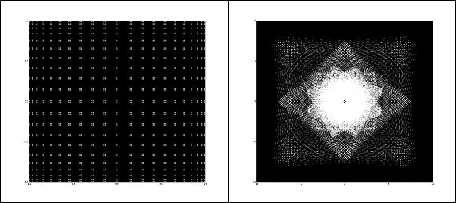
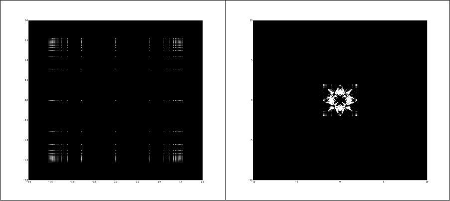
In the previous post, I showed the results of a complex division test where the original complex plane points are a lattice of points z=[-a,a]+[-a,a]i where a is an integer. Let us call L to the set of complex points z of this lattice. Those lattice points form a mesh of points in the complex plane. When the complex division is performed over the lattice (this means that every z complex number of L is divided by the rest of the points of L and itself) the result is a pattern that initially looks similar to some quasicrystal diffraction patterns (please see my previous post for videos and plottings). Below, left side, the original complex plane lattice points and in the right side the pattern that is generated applying complex division over the lattice points as explained above. These examples are made for a lattice L whose value a is 41, so z=[-41,41]+[-41,41]i. This means that the original lattice L is including 83x83 = 6889 complex numbers.

I wanted to know how the transformation of the original lattice modified the resulting pattern, so I have started to test the trigonometric functions applied to the original lattice points. The results are also quite amazing. Here is a briefing about it:

1. Transformation of the complex numbers z of L as follows: z=sin([-a,a])+sin([-a,a])i. Left side, the result of the transformation of L and in the right side the pattern that is generated.

Here is a video zooming in and out the pattern:

2. Transformation of the complex numbers z of L as follows: z=cos([-a,a])+cos([-a,a])i. Left side, the result of the transformation of L and in the right side the pattern that is generated.

It is a little bit similar to the sine transformation, but it is not identical. It is possible also to make hybrids of sine and cosine functions and the resulting patterns are variations of the patterns shown above.

Here is a video zooming in and out the pattern:

3. Transformation of the complex numbers z of L as follows: z=cosec([-a,a])+cosec([-a,a])i. Left side, the result of the transformation of L and in the right side the pattern that is generated.

Here is a video zooming in and out the pattern:

4. Transformation of the complex numbers z of L as follows: z=cotan([-a,a])+cotan([-a,a])i. Left side, the result of the transformation of L and in the right side the pattern that is generated. 

Here is a video zooming in and out the pattern:

5. Transformation of the complex numbers z of L as follows: z=arctan([-a,a])+arctan([-a,a])i. Left side, the result of the transformation of L and in the right side the pattern that is generated.

Here is a video zooming in and out the pattern:

Some of the trigonometric transformations look similar, but they are not exactly the same patterns. These are some zoomed plottings of them:

1. Sine pattern:

2. Cosine pattern:

 3. Cosecant pattern:

4. Cotangent pattern:

5. Arctangent pattern:

Finally, here are some plottings of the closest points to 0+0i, from left to right, top-down, cosine, sine, cosecant, cotangent, tangent, secant. The cosine and sine, cosecant and secant and cotangent and tangent patterns look similar:

I am still testing some other transformations of the original lattice L, but initially they are not so interesting. I will post them in a former post. Some days ago Terence Tao posted an article named "Sweeping a matrix rotates its graph" explaining the technique named "Sweeping" performed over squared matrices which is also based on division by selecting a pivot point of the main diagonal of the matrix. I will try to use that technique setting up the lattice L as a matrix of complex numbers and see what happens, the results could be a variation of these ones. If somebody reading this knows more about these type of patterns please let me know to share ideas.

Some random plottings

The plottings on this post are only for reference in other places like LinkedIn or MSE.

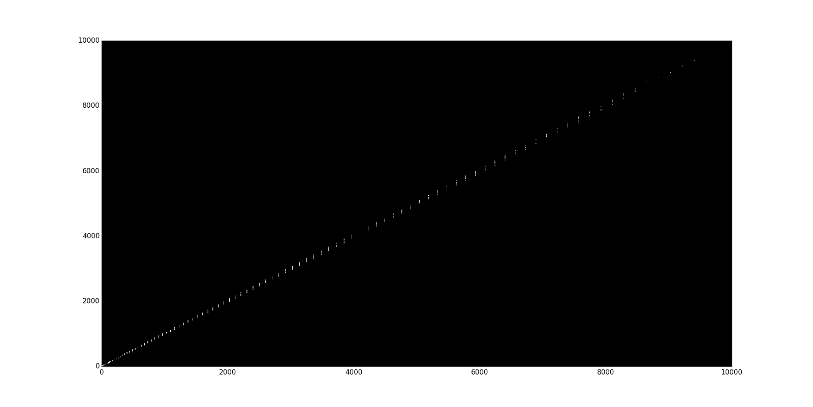
1. Plotting of the sequence S = {p(n)^p(n+1) mod (p^n+2)} where x=trunc(sqrt(s(i))) and y=s(i)-(x^2): 

How to plot the Gamma function fractal

The Gamma function is an extension of the factorial (n!) function, with its argument shifted down by 1, to real and complex numbers. And there is a fractal associated to it. I just wanted to learn how to make it because I want to learn how to plot the Mandelbrot set, and the Gamma function fractal seems easier to catch the idea of recursion. So here is how to make it!

First of all, I have been following the great explanation at Mathistopheles website, but I needed to study by myself some details to make it work properly.  

Basically, when the gamma function is calculated for a complex number z repeatedly (nested, and shifting down 1 the complex number according to the definition), this is: Gamma(Gamma(...(Gamma(z-1)...-1)-1), the final value result of the nested calculations either tends to 1 or grows without limit. So it is possible to map each z (=a+bi) value of the complex plane (in Cartesian coordinates) with a color code showing if the value tends to 1 (this the same as saying that it tends to the complex number 1+0i) or not in a specific numbers of calculations of the nested Gamma function. 

The condition to tend to 1 is as follows: let us say we want to know if the nested calculation of the Gamma function applied to z = (a+bi) tends to 1. In a first step, calculate Gamma(z-1) = c+di. If the distance of the real part a to 1 is greater or equal to the distance of c to 1 and the absolute value of the imaginary part b is greater than the absolute value of the imaginary part d (abs(b)>=abs(d)) then it is possible to say that z tends to 1+0i when the Gamma function is applied over z (nested as it was explained above). 

It is important to understand that it can happen that the first calculation for a given complex number z1 of Gamma(z1-1) provides a complex number z2 which is not closer to 1 than the original z1. And that does not mean that z1 does not tend to 1 when the nested Gamma function is applied again to z2. It could happen that when Gamma(z2-1) = z3 is calculated, z3 is closer to 1 than z2, and in the moment that this happens then the result is that from that point z1 tends to 1 when the nested calculations are applied. So sometimes we just need one calculation of Gamma for the initial complex number z1 to know if it tends to 1 and sometimes we need two nested Gamma calculations, sometimes 3, 4, 5, ... etc sometimes hundreds or thousands. But the calculation of the computer is very slow when the Gamma function is applied hundreds of times for each complex number, so usually a limit of for instance 7 nested Gamma calculations is applied to decide if a complex number tends to 1 or not. It is not totally accurate, but good enough to start to see the fractal patterns of the Gamma function. The more nested calculations the more accurate the patterns will be, and of course, the more complex numbers are calculated, the more we can zoom into the fractal pattern. 

And here is the result:

It is the typical image of the Gamma fractal function in the complex plane interval [-5,0]+[-1,1]i. I tried to find a good combination of colors. The complex numbers that tend to 1 in just one Gamma calculation are in black color. Then Dark blue two nested calculations, then Pink... finally up to Yellow (7 nested loops). The complex numbers that do not tend to 1 in less than 8 nested calculations are in the Blue color (if the reader can rememeber the good old Fractint, it was the popular color used for that purpose!).

Just to finish here is another version in polar coordinates:

And here is the Python code, modifying the value of the "method" variable it is possible to render Cartesian, Polar or Spherical coordinates. Use it freely:

def gamma_fractal():
    import matplotlib.pyplot as plt
    from scipy.special import gamma
    from numpy import real, imag, around, arange, float, cos, sin, pi

    import matplotlib as mpl

    from mpl_toolkits.mplot3d import Axes3D

   
    #0 Cartesian, 1 Polar, 3 Spherical
    method = 0

    if method==3:
        mpl.rcParams['legend.fontsize'] = 10


        fig = plt.figure()

        ax = fig.gca(projection='3d')
       
    arraydim = 1000000
    xrange = [arange(arraydim,dtype=float),arange(arraydim,dtype=float),arange(arraydim,dtype=float),arange(arraydim,dtype=float),arange(arraydim,dtype=float),arange(arraydim,dtype=float),arange(arraydim,dtype=float),arange(arraydim,dtype=float)]
    yrange = [arange(arraydim,dtype=float),arange(arraydim,dtype=float),arange(arraydim,dtype=float),arange(arraydim,dtype=float),arange(arraydim,dtype=float),arange(arraydim,dtype=float),arange(arraydim,dtype=float),arange(arraydim,dtype=float)]
    zrange = [arange(arraydim,dtype=float),arange(arraydim,dtype=float),arange(arraydim,dtype=float),arange(arraydim,dtype=float),arange(arraydim,dtype=float),arange(arraydim,dtype=float),arange(arraydim,dtype=float),arange(arraydim,dtype=float)]
    hexcolor=["#000000","#131667","#F028B3","#42677C","#3EA670","#6DD02D","#F9B90F","#0000FF"]
    pos=[0,0,0,0,0,0,0,0]
   
    ival = 0+1j

    if method!=3:
        firstx = -5
        lastx = 0
        firsty = -1
        lasty = 1
        incx = 0.0005
        incy = 0.0005
    else:
        firstx = -pi
        lastx = pi
        firsty = -pi
        lasty = pi
        incx = 0.002
        incy = 0.002
    posx = firstx
   
   
    while posx < lastx:
        posy = firsty
        while posy < lasty:
            counter = 0           
            mycomplex = gamma((posx+1)+(posy*ival))
            nextcomplex = gamma(mycomplex+1)

            while counter < 7:
                if (abs(mycomplex.imag) > abs(nextcomplex.imag)) and (abs(1-mycomplex.real) > abs(1-nextcomplex.real)):
                    break
                mycomplex = nextcomplex
                nextcomplex = gamma(mycomplex+1)

                counter = counter + 1
           
            if method == 0:
                xrange[counter][pos[counter]] = posx
                yrange[counter][pos[counter]] = posy
            elif method == 1:
                xrange[counter][pos[counter]] = posx*cos(posy)
                yrange[counter][pos[counter]] = posx*sin(posy)
            else:
                xrange[counter][pos[counter]] = cos(posy)*cos(posx)
                yrange[counter][pos[counter]] = sin(posy)*cos(posx)
                zrange[counter][pos[counter]] = sin(posx)

            pos[counter] = pos[counter] + 1

            if pos[counter]==arraydim:
                newxrange = arange(pos[counter],dtype=float)       
                newyrange = arange(pos[counter],dtype=float)
                newzrange = arange(pos[counter],dtype=float)   

                for i in range(0,pos[counter]):
                    newxrange[i]=xrange[counter][i]
                    newyrange[i]=yrange[counter][i]
                    if method == 3:
                        newzrange[i]=zrange[counter][i]

                if method != 3:
                    plt.plot(newxrange,newyrange,",",color=hexcolor[counter])
                else:
                    ax.plot(newxrange, newyrange, newzrange,",",color=hexcolor[counter])


                pos[counter]=0
           
            posy = posy + incy
        posx = posx + incx

    for c in range (0,8):
        newxrange = arange(pos[c],dtype=float)       
        newyrange = arange(pos[c],dtype=float)       
        newzrange = arange(pos[c],dtype=float)   
        for i in range(0,pos[c]):
            newxrange[i]=xrange[c][i]
            newyrange[i]=yrange[c][i]
            if method == 3:
                newzrange[i]=zrange[c][i]

        if method != 3:
            plt.plot(newxrange,newyrange,",",color=hexcolor[c])
        else:
            ax.plot(newxrange, newyrange, newzrange,",",color=hexcolor[c])

           
        pos[c]=0

    if method!=3:
        ax = plt.gca()
        ax.set_axis_bgcolor((0, 0, 0))
        figure = plt.gcf()
        figure.set_size_inches(30, 20)
        if method == 0:
            plt.axis([firstx,lastx,firsty,lasty])
        plt.savefig("gamma_"+str(method)+".png")
        plt.show()
    else:
        #ax.legend()
        #ax.dist=8
        for ii in range(0,361):
            ax.view_init(elev=-178., azim=ii)
            mpl.pyplot.savefig("movie"+str(ii)+".png")
        #ax.view_init(elev=28., azim=ii)
        #plt.show()


gamma_fractal()

Enjoy the fractals!

A very nice pattern based on Euler's identity

Euler's identity is one of the jewels of Mathematics, it blends in one sight some of the most significant constants of the mathematical universe:

I tried to visualize how would look the left part of the identity in the complex plane by using the following function:

It is a tryout of a generic version of the left side of Euler's identity. Applying the change e^{ib}=cos(b)+sin(b)i, the following function is obtained:

For instance, to be able to see the patterns, taking k1,k2,k3 in the interval [−10,10] stepping in by 0.1, and calculating all the possible combinations of triplets (k1,k2,k3) and their values f(k1,k2,k3), this is the pattern that it generates when the complex values a+bi are represented in Cartesian coordinates (a=x,b=y):

A closer approach to 0+0i:

Euler's identity f(1,1,1)=e^{pi*i}+1=0+0i would be located at the center and the rest of points are the closer values of the more generic function f(k1,k2,k3) as it was defined above for the example. As expected is periodic and symmetrical. This is a little video:

Isn't it hypnotic? I have asked at MSE about this pattern, as far as I know it might be the fist time that has been plotted. I hope somebody will be able to propose some insights about it!  

Update 2016/01/15: Professor Brent Yorgey kindly gave a very nice explanation of the pattern at MSE!