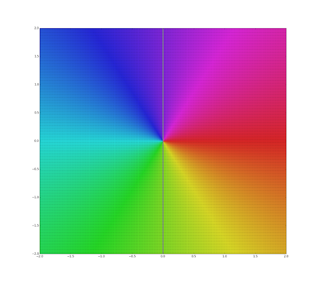
Recently I have made a question regarding the Complex Domain coloring technique at MSE.
Basically, as Wikipedia says:
"Domain coloring is a technique for visualizing functions of a complex variable ...There were many earlier uses of color to visualize complex functions, typically mapping argument (phase) to hue."
So basically I have learned how to do the basic hue map when we have a complex injective function $f(z)$. These are some simple examples:
$(1)\ f(z)=\frac{1}{z}$
$(1)\ f(z)=\frac{1}{z}$
$(2)\ f(z)=\frac{(z^2-1)(z-2-i)^2}{z^2+2+2i}$
$(3)\ f(z)=z^3+1$
$(4)\ f(z)=z^5-1$.
$(5)\ f(z)=e^z$.
They are the mappings we are used to see. But to my surprise, then I
tried a "reverse" mode, instead of mapping over the positions of the
input complex points (the domain of the function), mapped the output
points with the conversion to hue of the original input points, a kind
of "Range coloring" or "Image coloring" or "coloring map over the
result" of the function, the results were also very impressive. They are
the other side of the coin of the relationship between the Domain and
the Image/Range of the function (in the same order than before):

As usual, this is the Python code I have prepared to create the graphics. Feel free to use it and modify it:
def hsl_rgb_visu():
def hslToRgb(h, s, l):
# Source: https://stackoverflow.com/questions/2353211/hsl-to-rgb-color-conversion
# Converts an HSL color value to RGB. Conversion formula
# adapted from http://en.wikipedia.org/wiki/HSL_color_space.
# Assumes h, s, and l are contained in the set [0, 1] and
# returns r, g, and b in the set [0, 255].
def hue2rgb(p, q, t):
if t < 0:
t += 1
if t > 1:
t -= 1
if t < 1/6:
return p + (q - p) * 6 * t
if t < 1/2:
return q
if t < 2/3:
return p + (q - p) * (2/3 - t) * 6
return p
r,g,b = 0,0,0
if s == 0:
r,g,b = l,l,l
else:
q=0
if l < 0.5:
q=l * (1 + s)
else:
q=l + s - l * s
p = 2 * l - q;
r = hue2rgb(p, q, h + 1/3)
g = hue2rgb(p, q, h)
b = hue2rgb(p, q, h - 1/3)
prevR=str(hex(round(r * 255))).replace("0x","")
prevG=str(hex(round(g * 255))).replace("0x","")
prevB=str(hex(round(b * 255))).replace("0x","")
if len(prevR)==1:
prevR="0"+prevR
if len(prevG)==1:
prevR="0"+prevR
if len(prevB)==1:
prevR="0"+prevR
return "#"+prevR+prevG+prevB
from sympy import mobius, factorint, totient
from gmpy2 import is_prime, is_square
import matplotlib.pyplot as plt
import csv
from random import randint
from math import sqrt, log, cos , sin , tan, pi, atan2, acos, pi
import numpy as np
import cmath as cmath
import fractions
def lcm(a,b): return abs(a * b) / fractions.gcd(a,b) if a and b else 0
testlimit = 200
testbase = 100
lx=[]
ly=[]
lc=[]
lh=[]
ll=[]
lr=[]
ls=[]
print("Calculating...")
maxx=0
maxy=0
for posx in range(-testlimit,testlimit+1):
for posy in range(-testlimit,testlimit+1):
x=posx/testbase
y=posy/testbase
# Make function
# function indentity
#resx = x
#resy = y
#maxx = testlimit**2
#maxy = testlimit**2
# function complex multiplicative inverse 1/z example0
#myc=x+(y*(1j))
#if myc == 0:
# myc = 0
#else:
# myc=1/myc
# function complex example1
#myc=x+(y*(1j))
#myc=(((myc**2)-1)*(myc-2-(1j))**2)/((myc**2)+2+(2j))
# function complex example2
#myc=x+(y*(1j))
#myc=(myc**3)+1
# function complex z^5-1 example3
#myc=x+(y*(1j))
#myc=(myc**5)-1
# function complex exp, asin, atan, acos, sin, tan, cos (con h) example4
myc=x+(y*(1j))
myc=cmath.exp(myc)
resx=myc.real
resy=myc.imag
# Make the inverse mapping
#if abs(resx)>5 or abs(resy)>5:
# continue
# Make the inverse mapping
#tmpresx = resx
#tmpresy = resy
#resx=x
#resy=y
if abs(resx)>maxx:
maxx=abs(resx)
if abs(resy)>maxy:
maxy=abs(resy)
current_angle = 0
current_r = sqrt((resx**2)+(resy**2))
if resx!=0:
current_angle = atan2(resy,resx)
else:
if y>0:
current_angle = pi/2
else:
current_angle = (pi/2)*3
if current_angle < 0:
current_angle = current_angle + (2*pi)
current_angle = (1/(2*pi))*current_angle
h = current_angle
l = 0.5
s = 0.7
lx.append(x)
ly.append(y)
# Make the inverse mapping
#lx.append(tmpresx)
#ly.append(tmpresy)
lh.append(h)
ll.append(l)
ls.append(s)
lr.append(current_r)
base=1/(sqrt((maxx**2)+(maxy**2)))
for i in range(0,len(lx)):
#ls[i] = 0.88-(base*lr[i])
#ll[i] = 1-(1/(2**(1+(base*abs(lr[i])))))
lc.append(hslToRgb(lh[i], ls[i], ll[i]))
print("Plotting...")
ax = plt.gca()
ax.set_axis_bgcolor((0, 0, 0))
figure = plt.gcf()
figure.set_size_inches(18, 16)
for i in range(0,len(lx)):
print("Current index="+str(i)+" of "+str(len(lx)-1)+"\r", end='')
plt.plot(lx[i],ly[i],".",color=lc[i])
plt.savefig("visualize_4var_functions_with_colors.png")
#plt.show()
print("End...")
hsl_rgb_visu()
I think that in terms of Complex Domain coloring still there are things to explode and we are still seeing only one side of the coin. And the other side seems quite interesting!


No comments:
Post a Comment