Converting complex domain coloring visualizations into autostereograms

As Wikipedia says regarding the domain coloring technique for complex functions:

"A graph of a complex function $g : \Bbb C \to \Bbb C $ of one complex variable lives in a space with two complex dimensions. Since the complex plane itself is two-dimensional, a graph of a complex function is an object in four real dimensions. That makes complex functions difficult to visualize in a three-dimensional space. "

The domain coloring technique transforms the points belonging to $f(z)$ into hue, brightness and saturation values, all normalized into $[0,1]$. Usually the argument of the complex number $f(z)$ is converted into a normalized value $[0,1]$ and then associated to a hue value. Then the color associated to $f(z)$ is shown at the position $z$.

For instance, $f(z)=z^3+1$. This is how looks the interval $z=[+/-]4+[+/-]3i$:

So far so good. But we cannot perceive the sense of depth. So what I want to do is bringing up that depth using autostereograms.

My first idea was applying directly the normalized color map as depth map, and then create the autostereogram. The normalized color map shown above is converted into the following depth map:

And then it is possible to create the autostereogram. It is of the "wall-eyed" ("parallel") convergence type (non-cross eyed). The three-dimensional effect can be produced by both eyes looking at a the image by defocusing the eyes at a certain distance. The examples are fine-tuned to be seen at a distance around $30-40$cm (click in the image to see a full screen view):

There is a trick: it is included a subtle layer with the original color map, and then added transparency to the autostereogram (alpha=0.9). In that way, the original color map can be slightly seen and works as a color texture over the autostereogram, so when we look at it, we can see that colors and depth are matching.

Two more examples: $f(z)=z^5-1$ and $f(a+bi)=\tan{(ab)}+atan(ab)i$:

Indeed it is possible to make also animations once the eye gets used to the correct focal length. I wonder if this technique is in use (e.g. educational purposes). Initially it seems very interesting! I have added a question at MSE regarding this topic.

Complex Domain coloring vs Complex Range (over the output) coloring: which one brings more information?

Recently I have made a question regarding the Complex Domain coloring technique at MSE.

Basically, as Wikipedia says: 

"Domain coloring is a technique for visualizing functions of a complex variable ...There were many earlier uses of color to visualize complex functions, typically mapping argument (phase) to hue."

So basically I have learned how to do the basic hue map when we have a complex  injective function $f(z)$. These are some simple examples:

$(1)\ f(z)=\frac{1}{z}$ 

$(2)\ f(z)=\frac{(z^2-1)(z-2-i)^2}{z^2+2+2i}$

$(3)\ f(z)=z^3+1$ 

$(4)\ f(z)=z^5-1$.

$(5)\ f(z)=e^z$.

They are the mappings we are used to see. But to my surprise, then I tried a "reverse" mode, instead of mapping over the positions of the input complex points (the domain of the function), mapped the output points with the conversion to hue of the original input points, a kind of "Range coloring" or "Image coloring" or "coloring map over the result" of the function, the results were also very impressive. They are the other side of the coin of the relationship between the Domain and the Image/Range of the function (in the same order than before): 

As usual, this is the Python code I have prepared to create the graphics. Feel free to use it and modify it:

def hsl_rgb_visu():

    def hslToRgb(h, s, l):
        # Source: https://stackoverflow.com/questions/2353211/hsl-to-rgb-color-conversion
        # Converts an HSL color value to RGB. Conversion formula
         # adapted from http://en.wikipedia.org/wiki/HSL_color_space.
         # Assumes h, s, and l are contained in the set [0, 1] and
         # returns r, g, and b in the set [0, 255].
        def hue2rgb(p, q, t):
            if t < 0:
                t += 1
            if t > 1:
                t -= 1
            if t < 1/6:
                return p + (q - p) * 6 * t
            if t < 1/2:
                return q
            if t < 2/3:
                return p + (q - p) * (2/3 - t) * 6
            return p
      
        r,g,b = 0,0,0

        if s == 0:
            r,g,b = l,l,l
        else:
            q=0
            if l < 0.5:
                q=l * (1 + s)
            else:
                q=l + s - l * s
              
            p = 2 * l - q;
            r = hue2rgb(p, q, h + 1/3)
            g = hue2rgb(p, q, h)
            b = hue2rgb(p, q, h - 1/3)
      
        prevR=str(hex(round(r * 255))).replace("0x","")
        prevG=str(hex(round(g * 255))).replace("0x","")
        prevB=str(hex(round(b * 255))).replace("0x","")
      
        if len(prevR)==1:
            prevR="0"+prevR
        if len(prevG)==1:
            prevR="0"+prevR
        if len(prevB)==1:
            prevR="0"+prevR
          
        return "#"+prevR+prevG+prevB
      
    from sympy import mobius, factorint, totient
    from gmpy2 import is_prime, is_square
    import matplotlib.pyplot as plt
    import csv
    from random import randint
    from math import sqrt, log, cos , sin , tan, pi, atan2, acos, pi
    import numpy as np
    import cmath as cmath
    import fractions
   
    def lcm(a,b): return abs(a * b) / fractions.gcd(a,b) if a and b else 0
   
    testlimit = 200
    testbase = 100
   
    lx=[]
    ly=[]
    lc=[]
   
    lh=[]
    ll=[]
    lr=[]
    ls=[]
   
    print("Calculating...")
    maxx=0
    maxy=0
    for posx in range(-testlimit,testlimit+1):
        for posy in range(-testlimit,testlimit+1):
      
            x=posx/testbase
            y=posy/testbase
          
            # Make function
          
            # function indentity
            #resx = x
            #resy = y
            #maxx = testlimit**2
            #maxy = testlimit**2
          
            # function complex multiplicative inverse 1/z example0
            #myc=x+(y*(1j))
            #if myc == 0:
            #    myc = 0
            #else:
            #    myc=1/myc
          
          
            # function complex example1
            #myc=x+(y*(1j))
            #myc=(((myc**2)-1)*(myc-2-(1j))**2)/((myc**2)+2+(2j))
          
            # function complex example2
            #myc=x+(y*(1j))
            #myc=(myc**3)+1
          
            # function complex z^5-1 example3
            #myc=x+(y*(1j))
            #myc=(myc**5)-1
          
            # function complex exp, asin, atan, acos, sin, tan, cos (con h) example4
            myc=x+(y*(1j))
            myc=cmath.exp(myc)
          
            resx=myc.real
            resy=myc.imag
          
            # Make the inverse mapping
            #if abs(resx)>5 or abs(resy)>5:
            #    continue
          
            # Make the inverse mapping
            #tmpresx = resx
            #tmpresy = resy
            #resx=x
            #resy=y
          
          
            if abs(resx)>maxx:
                maxx=abs(resx)
            if abs(resy)>maxy:
                maxy=abs(resy)
          
            current_angle = 0
            current_r = sqrt((resx**2)+(resy**2))
            if resx!=0:
                current_angle = atan2(resy,resx)
            else:
                if y>0:
                    current_angle = pi/2
                else:
                    current_angle = (pi/2)*3
              
            if current_angle < 0:
                current_angle = current_angle + (2*pi)
          
            current_angle = (1/(2*pi))*current_angle
              
            h = current_angle
            l = 0.5
            s = 0.7
          
            lx.append(x)
            ly.append(y)
          
            # Make the inverse mapping
            #lx.append(tmpresx)
            #ly.append(tmpresy)
          
            lh.append(h)  
            ll.append(l)  
            ls.append(s)
            lr.append(current_r)  
          
    base=1/(sqrt((maxx**2)+(maxy**2)))
    for i in range(0,len(lx)):
        #ls[i] = 0.88-(base*lr[i])
        #ll[i] = 1-(1/(2**(1+(base*abs(lr[i])))))
        lc.append(hslToRgb(lh[i], ls[i], ll[i]))
          
    print("Plotting...")
    ax = plt.gca()
    ax.set_axis_bgcolor((0, 0, 0))
    figure = plt.gcf()
    figure.set_size_inches(18, 16)
    for i in range(0,len(lx)):
        print("Current index="+str(i)+" of "+str(len(lx)-1)+"\r", end='')
        plt.plot(lx[i],ly[i],".",color=lc[i])
    plt.savefig("visualize_4var_functions_with_colors.png")
    #plt.show()
    print("End...")
   
hsl_rgb_visu()

I think that in terms of Complex Domain coloring still there are things to explode and we are still seeing only one side of the coin. And the other side seems quite interesting!

How to build a projection (Schlegel diagram) of a tesseract, and show a four-dimensional point inside it (II)

Some months ago I described in a post how to build a projection (Schlegel diagram) of a tesseract, and show a four-dimensional point inside it. Since then I have used it to review the symmetries of $(w,x,y,z,)$ four-dimensional tuples by observing the $3D$ projection of the cloud of points. 

Recently I have been able to use it for a real problem of a MSE user. Here is the link to the question. I am really happy to have been useful to somebody else. This are two of the projections of the more than $4 \cdot 10^4$ four-dimensional cloud of points of the problem. They look gorgeous!

$(w, x, $Shadow of plane$(y,z))$:

 

$($Shadow of plane$(w,x), y, z)$:

Hobbymath's wanderings #18

Spouge's_approximation (Wiki).

Lanczos_approximation (Wiki).

Proof of the Euler product formula for the Riemann zeta function (Wiki).

Birds and Frogs (Freeman Dyson's article).

Wolstenholme's theorem (Wiki).

Lenstra elliptic curve factorization (Wiki).

Lambert W function (Wiki).

Arithmetic derivative (Wiki).

Cartessian Genetic Programming (pdf).

Cartessian Genetic Programming.

Cartessian Genetic Programming (resources).

Hardy&Littlewood circle method (Wiki).

Dedekind eta function (Wiki).

Modular form (Wiki).

Modular_group (Wiki).

Wallis product (Wiki).

Proof_by_infinite_descent: Irrationality of sqrt(2) (Wiki).

A mathematicians's miscellany (Littlewood)

"I once challenged Hardy to find a misprint on a certain page of a joint paper: he failed. It was in his own name : 'G,H.Hardy'."

"Schoolmaster : 'Suppose x is the number of sheep in the problem'. Pupil: 'But, Sir, suppose x is not the number of sheep'. [I asked Prof. Wittgenstein was this not a profound philosophical joke, and he said it was.]"

("A Mathematician's Miscellany", J.E.Littlewood, 1953)

Trying to refine Ingham's prime gap expression

Sometimes it is difficult to get feedback about a calculation or the steps of a proof. This is one of those cases. This is a mirror of my question at MSE.

Let $p_n$ denote the $n^{th}$ prime number. Ingham showed that:
$$p_{n+1} - p_n \lt K p_n^{\frac{5}{8}}$$
where $K$ is a fixed positive integer, is an upper bound for the prime gaps.

(A.E.Ingham, On the difference between consecutive primes, Quart. J. Math. Oxford Ser. vol. 8 (1937) pp. 255-266)

I am trying to know if the following manipulations would be valid to reduce the value $\frac{5}{8}$ up to $\frac{1}{8}$. The steps $1,2,3$ have been verified in, but still I am trying to get some help to review the rest of them.

1. Both sides to the eighth: $$(p_{n+1} - p_n)^8 \lt K^8 p_n^{5}$$
2. Def. $K_2 = K^8$ a new fixed constant $K_2 \gt K$: $$(p_{n+1} - p_n)^8 \lt K_2 p_n^{5}$$
3. By Fermat's Little Theorem, we know that $p_n^{5}$ can be replaced as follows}: $$p_n^{5}= 5K^{'} + p_n$$
For a given positive unbounded constant $K^{'}$. Thus: $$(p_{n+1} - p_n)^8 \lt K_2 (5K^{'} + p_n)$$
But (credits for the following explanation to a MSE user here) the map $$ K' : \mathbb{P} \to \mathbb{N} : p \mapsto \frac{p^5 - p}{5}$$
is not constant and unbounded from above.

$\color{red}{From\ this\ point\ ahead\ the\ manipulations\ need\ to\ be\ verified}$.

The right side of the inequality can be replaced as follows: $$(p_{n+1} - p_n)^8 \lt K_2 (5K^{'} + p_n) = (K_2 \cdot 5K^{'}) + K_2 p_n$$
Our partial refinement will be true only if the constants are fixed, so we need to add a condition to handle the unbounded constant $(K_2 \cdot 5K^{'})$. So let us assume the following condition:

Condition 1: $$ p_n^{5}-p_n = 5K^{'} \lt K_2 = K^8$$

So from now on, the partial refinement will be valid only those primes $p_n$ whose value $p_n^{5}-p_n$ is bounded by the eighth power of Ingham's $K$ constant.

4. Def. $K_3 = K_2^2$ an even bigger new fixed constant $K_3 \gt K_2$: $$(p_{n+1} - p_n)^8 \lt K_3 + K_2 p_n$$
5. As $K_3 \gt K_2$, it is also true that: $$(p_{n+1} - p_n)^8 \lt K_3 + K_2 p_n  \lt K_3 + K_3 p_n = K_3 (1+p_n) \lt K_3 (2p_n) = (2K_3)p_n$$
6. Def. $K_4 = 2K_3$ as an even bigger new fixed constant $K_4 \gt K_3$: $$(p_{n+1} - p_n)^8 \lt K_4p_n$$
7. Now we make again the $8^{th}$ root in both sides: $$p_{n+1} - p_n \lt K_4^{\frac{1}{8}}p_n^{\frac{1}{8}}$$
8. Finally, def. $K_5 = K_4^{\frac{1}{8}}$ as a new fixed constant. In this case $K_5 \lt K_4$ but still fixed and positive: $$p_{n+1} - p_n \lt K_5p_n^{\frac{1}{8}}$$
Only valid under Condition 1: $$ p_n^{5}-p_n \lt K^8$$
being $K$ the original Ingham's $K$ constant.

Thus, if the manipulations and redefinition of constants are correct:

1. If $ p_n^{5}-p_n \lt K^8$: $$p_{n+1} - p_n \lt K_5 p_n^{\frac{1}{8}} = 2^{\frac{1}{8}}K^2 p_n^{\frac{1}{8}}$$
for a fixed constant $K_5 = K_4^{\frac{1}{8}}=(2K_3)^{\frac{1}{8}}=(2K_2^2)^{\frac{1}{8}}=(2(K^8)^2)^{\frac{1}{8}}=2^{\frac{1}{8}}K^2$, and

2. In the rest of unbounded cases remains as the original Ingham's expression: $$p_{n+1} - p_n \lt K p_n^{\frac{5}{8}}$$
I have asked at MSE if this is correct or not, and if it is useful or not. If it is correct, is just valid for a finite range of prime numbers $p_n=2,3,5...$ as long as $ p_n^{5}-p_n \lt K^8$. If I receive an answer I will write here the results too.

Are quaternions useful as coordinate systems for two-dimensional manifolds?

This is complementary information about my question at MSE "Are quaternions useful as coordinate systems for two-dimensional manifolds?" that I cannot add there due to the weight of the images and the length of the question. 

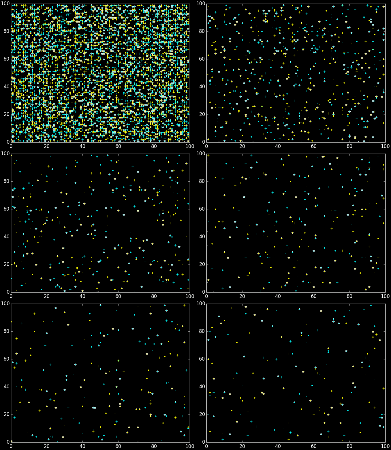
 This is the evolution of the first 500 steps of a test:

Same with some motion blur (basically is just a visualization test):

This is the Python code, please use and modify it freely:

 def quat():
    from sympy import mobius, factorint, totient
    from gmpy2 import is_prime, is_square
    import matplotlib.pyplot as plt
    import csv
    from random import randint
    from math import sqrt, log, cos , sin , tan, pi
  
    test_n_limit = 7000
    test_loop_limit = 500
    loa = []
    loi = []
    loj = []
    lok = []
    A=2
    I=100
    J=100
    K=4
      
    # Generating first positions of the elements
    for n in range (0,test_n_limit):
        loa.append(randint(0,A-1))
        loi.append(randint(0,I-1))
        loj.append(randint(0,J-1))
        lok.append(randint(0,K-1))
  
    for i in range(0,test_loop_limit):
        nloa = []
        nloi = []
        nloj = []
        nlok = []
        removed=[]
        for n in range (0,len(loa)):
            if n in removed:
                continue
            collided=False
            for m in range (n+1,len(loa)):
                if m in removed:
                    continue
                if loa[n]==loa[m] and loi[n]==loi[m] and loj[n]==loj[m] and lok[n]==lok[m]:
                    collided = True
                    removed.append(m)
                    # The collision produces a new point generated by a quaternion sum and the former points dissapear
                    nloi.append((loi[n]+loi[m])%I)
                    if (loi[n]+loi[m] >= I):
                        # The point goes out of the surface from the right, so it goes to the other side of the Mobius band
                        nloa.append((loa[n]+1)%A)
                        nloj.append(J-1-((loj[n]+loj[m])%J))
                    else:
                        nloa.append(loa[n])
                        nloj.append((loj[n]+loj[m])%J)
                    nlok.append((lok[n]+lok[m])%K)
                  
                elif loi[n]==loi[m] and loj[n]==loj[m] and lok[n]==lok[m]:
                    collided = True
                    removed.append(m)
                    # The collision produces a new point generated by a Hamiltonian product and the former points dissapear
                    nloa.append(((loa[n]*loa[m])-(loi[n]*loi[m])-(loj[n]*loj[m])-(lok[n]*lok[m]))%A)
                    nloi.append(((loa[n]*loi[m])+(loi[n]*loa[m])+(loj[n]*lok[m])-(lok[n]*loj[m]))%I)
                    nloj.append(((loa[n]*loj[m])-(loi[n]*lok[m])+(loj[n]*loa[m])+(lok[n]*loi[m]))%J)
                    nlok.append(((loa[n]*lok[m])+(loi[n]*loj[m])-(loj[n]*loi[m])+(lok[n]*loa[m]))%K)
                  
            if collided==False:
                # A collision did not happen and the point moves in a random walk
                incx = randint(-1,1)
                incy = randint(-1,1)
              
                nloi.append((loi[n]+incx)%I)
                if (loi[n]+incx >= I) or (loi[n]+incx < 0):
                    # The point goes out of the surface from the right or left, so it goes to the other side of the Mobius band
                    nloa.append((loa[n]+1)%A)
                    nloj.append(J-1-((loj[n]+incy)%J))
                else:
                    nloa.append(loa[n])
                    nloj.append((loj[n]+incy)%J)
                nlok.append(lok[n])
              
        print_up_i_0=[]
        print_up_j_0=[]
        print_down_i_0=[]
        print_down_j_0=[]
        print_up_i_1=[]
        print_up_j_1=[]
        print_down_i_1=[]
        print_down_j_1=[]
        print_up_i_2=[]
        print_up_j_2=[]
        print_down_i_2=[]
        print_down_j_2=[]
        print_up_i_3=[]
        print_up_j_3=[]
        print_down_i_3=[]
        print_down_j_3=[]
        for n in range (0,len(loa)):
            if loa[n]==0:
                if lok[n]==0:
                    print_up_i_0.append(loi[n])
                    print_up_j_0.append(loj[n])
                elif lok[n]==1:
                    print_up_i_1.append(loi[n])
                    print_up_j_1.append(loj[n])
                elif lok[n]==2:
                    print_up_i_2.append(loi[n])
                    print_up_j_2.append(loj[n])
                elif lok[n]==3:
                    print_up_i_3.append(loi[n])
                    print_up_j_3.append(loj[n])
              
            else:
                if lok[n]==0:
                    print_down_i_0.append(loi[n])
                    print_down_j_0.append(loj[n])
                elif lok[n]==1:
                    print_down_i_1.append(loi[n])
                    print_down_j_1.append(loj[n])
                elif lok[n]==2:
                    print_down_i_2.append(loi[n])
                    print_down_j_2.append(loj[n])
                elif lok[n]==3:
                    print_down_i_3.append(loi[n])
                    print_down_j_3.append(loj[n])
      
        # Draw current status
        print_up_i_0.append(0)
        print_up_j_0.append(0)
        print_up_i_0.append(I)
        print_up_j_0.append(J)
        plt.plot(print_up_i_0,print_up_j_0,"b,")
        plt.plot(print_down_i_0,print_down_j_0,"r,")
        plt.plot(print_up_i_1,print_up_j_1,"b.")
        plt.plot(print_down_i_1,print_down_j_1,"r.")
        plt.plot(print_up_i_2,print_up_j_2,"b*")
        plt.plot(print_down_i_2,print_down_j_2,"r*")
        plt.plot(print_up_i_3,print_up_j_3,"b+")
        plt.plot(print_down_i_3,print_down_j_3,"r+")
        #plt.show()
        #figure.set_size_inches(18, 16)
        plt.savefig("Topology_MobiusBand_quaternion_"+str(i)+".png")
        plt.clf()
      
        loa=nloa
        loi=nloi
        loj=nloj
        lok=nlok

quat()